University of Manchester | 3rd Year Laboratory
While in Sections 2 and 3 we have explored some properties of the pulsar that did not require too much knowledge about the puslar itself, here we focus more on these aspects.
Known pulsars emit short pulses of electromagnetic radio waves with pulse periods between 1.4 ms and 8.5 s. Their radio emission is actually continuous but beamed, so any one observer sees a pulse of radiation each time the beam sweeps across his line-of-sight. Since the pulse periods equal the rotation periods of spinning neutron stars, they are quite stable. Even though the radio emission mechanism is not well understood, radio observations of pulsars have yielded a number of important results because:
Neutron stars are physics laboratories providing extreme conditions (deep gravitational potentials, densities exceeding nuclear densities, magnetic field strengths as high as B1014 or even 1015 gauss) not available on Earth.
Pulse periods can be measured with accuracies approaching 1 part in 1016, permitting exquisitely sensitive measurements of small quantities such as the power of gravitational radiation emitted by a binary pulsar system or the gravitational perturbations from planetary-mass objects orbiting a pulsar.
Before pulsars were discovered, astronomers were used to slowly varying or pulsating emission from stars, where the natural period was usually days. There is a lower limit to the rotation period $P$ of a gravitationally bound star, set by the requirement that the centrifugal acceleration at its equator not exceed the gravitational acceleration:
\begin{equation} \Omega^2 R < \frac{GM}{R^2} \end{equation}
where $\Omega$ is the angular velocity of the star, $R$ is its radius, $M$ its mass and $G$ the gravitational constant. Therefore, if a star rotates with angular velocity $\Omega = 2 \pi /P$, then \begin{equation} P^2 > \bigg( \frac{4\pi R^3}{3} \bigg )\frac{3\pi}{GM} \end{equation} and we can have a lower limit on its period. Furthermore, this can be re-written in terms of density as
\begin{equation} \boxed{\rho > \frac{3\pi}{GP^2}} \end{equation}
The fastest known pulsar had $P = 1.4\times 10^{-3}$ s, which implies a density limit of $\rho > 10^{14}$ g cm$^{-3}$, the density of nuclear matter. Consider a star of mass greater than Chandrasekhar mass $M_\mathrm{ch} \approx 1.4 M_\mathrm{sun}$, the maximum radius of this star would be
\begin{equation} R < \bigg ( \frac{3M}{4\pi\rho} \bigg )^{1/3}. \end{equation}
In the case of the pulsar with $P = 1.4 \times 10^{-3}$ and $\rho > 10^{14}$ g cm$^{-3}$,
\begin{equation} R < \bigg ( \frac{3\times 1.4 \times 2.0 \times 10^{33} \mathrm{g}}{4\pi \times 10^{14} \mathrm{g cm^{-3}}} \bigg )^{1/3} \approx 20 \mathrm{km} \end{equation} which is an order of magnitude apporximation to the radius of a pulsar and is used in the magnetic field calculations. The canonical neutron star is defined to have $M \approx 1.4 M_\mathrm{sun}$ and $R \approx 10$ km.
The Sun and many other stars are known to possess roughly dipolar magnetic fields. Stellar interiors are mostly ionized gas and hence good electrical conductors. Charged particles are constrained to move along magnetic field lines and, conversely, field lines are tied to the particle mass distribution. When the core of a star collapses from a size $10^11$ cm to $10^6$ cm, its magnetic flux is conserved and the initial magnetic field strength is multiplied by $10^10$, the factor by which the cross-sectional area falls. An initial magnetic field strength of $B \approx 100$ G becomes $B \approx 10^12$ G after collapse, so young neutron stars should have very strong dipolar fields. If the magnetic dipole of such a neutron star is inclined by some angle $\alpha > 0$ from the rotation axis, it emits low-frequency electromagnetic radiation. The Larmor formula for the power from an electric dipole is: \begin{equation} P_\mathrm{rad} = \frac{2q^2dot{\nu}^2}{3c^3} = \frac{2(q\ddot{r}\mathrm{sin}\alpha)^2}{3c^3} = \frac{2(\ddot{p_{\perp}})^2}{3c^3} \end{equation} where $p_\perp$ is the perpendicular component of the electric dipole moment. By analogy, the magnetic dipole radiation from an inclined dipole is \begin{equation} \boxed{P_\mathrm{rad} = \frac{2(\ddot{m_\perp})}{3c^3}} \end{equation} where $m_\perp$ is the perpendicular component of the magnetic dipole moment. For a uniformly magnetized sphere with radius $R$ and surface magnetic field strangth B, the magnetic diple memnt is $m = BR^3$. If the inclined dipole rotates with angular velocity $\Omega$, then \begin{equation} \ddot{m} = \Omega ^2 m_0 \mathrm{exp}(-i\Omega t) = \Omega ^2 m \end{equation} and hence, the power can be expressed as \begin{equation} P_\mathrm{rad} = \frac{2}{3c^3}(BR^3\mathrm{sin}\alpha)^2\bigg ( \frac{2\pi}{P} \bigg )^4 \end{equation} where we have expressed $\Omega$ in terms of the pulsar period $P$. This electromagnetic radiation will appear at the very low frequency < 1 kHz. This is so low that it cannot be observed because it does not propagate through the ionized Inter-Stellar Medium. The large power radiated is responsible for pulsar slowdown as it extracts rotational kinetic energy from the neutron star. The absorbed radiation can also light up a surrounding nebula, the Crab nebula for example.
The rotational kinetic energy $E_\mathrm{rot}$ is related to the moment of inertia $I$ by \begin{equation} E_\mathrm{rot} = \frac{1}{2}I\Omega ^2 = \frac{2\pi ^2 I}{P^2} \end{equation} and thus the moment of inertia for the canonical pulsar can be calculated, giving \begin{equation} \boxed{I = \frac{2}{5}MR^2 \approx 10^{30} \hspace{0.1cm} \mathrm{kg m^2}} \end{equation}
The pulsars that we obesrve today are slowing down gradually (i.e. period derivative is larger than 0). From the obesrved period and period derivative, one can estimate the rate at which the rotational energy is decreasing. By using Equation (10), we obtain \begin{equation} \frac{dE_\mathrm{rot}}{dt} = \frac{-4\pi^2 I \dot{P}}{P^3} \end{equation}
If we use the Equation (10) to estimate $P_\mathrm{rad}$, we can invert Larmor’s formula for magnetic dipole radiation to get a lower limit on the surface magnetic field strength, since one does not generally know the inclination angle $\alpha$. By equating expressions (9) and (12) and doing some algebra, one arrives at \begin{equation} B > \bigg( \frac{3c^3 I}{8\pi^2 R^6}P\dot{P} \bigg ) \end{equation}
If $B \mathrm{sin}\alpha$ does not change significantly with time, we can estimate a pulsar’s age $\tau$ from $P\dot{P}$ by assuming that the pulsar’s initial period $P_0$ was much shorter than the current period. Re-expressing Equation (13), this time with an equal sign, gives \begin{equation} P\dot{P} = \frac{8\pi^2 R^6 (B\mathrm{sin}\alpha)^2}{3c^3 I} \end{equation} that does not change with time. Considering that $PdP = P \dot{P}dt$ and integrating over the pulsar’s lifetime gives \begin{equation} \int_{P_0}^{P} PdP = \int_0^\tau P\dot{P}dt = P\dot{P}\int_0^\tau dt \end{equation}
since $P\dot{P}$ is assumed to be constant over time. Therefore, \begin{equation} \frac{P^2 - P_0^2}{2} = P\dot{P}\tau \end{equation} and the characteristic age, assuming that $P_0^2 \ll P^2$, is \begin{equation} \boxed{A = \frac{P}{2\dot{P}}} \end{equation} which is a good approximation for the actual age.
The ToAs of a pulsar were obtained from finding the differences between the observed data and a template. This was done by using the software PSRCHIVE the command
pat -f tempo2 -A SIS -F -t -s templatefile datafile
giving us the times of arrival of all the pulses measured followed by an error in microseconds. The template for the Crab pulsar was made available prior to the beginning of the experiments. However, ToAs were also determined for other pulsars.
To obtain the missing templates, we fitted a Von Mises distribution over the observed pulse to create a model by using paas -i and choosing the peak, width and height of the distribution manually. The model that was created this way was used as a template to determine the ToAs of the other pulsars using the same command mentioned above. Slider 2.1 shows every template used.


However, one wants to receive the pulse train from the pulsar at a relatively fixed point. Such a point is the barycenter of our solar system. We can switch reference frames if we know the extra time light would take to reach the barycenter rather the telescope at Jodrell Bank. Hence, each ToA will correspond to a delayed ToA at the barycenter. These latter ToAs can be calculated by adding the Earth Delay and the barycenter delay to the former ToAs.
A table with the barycenter position with respect to the Earth at midnight of every day in 2018 was available. Our observations did not always take place at midnight so interpolation was required. The chosen method was Lagrangian interpolation, using scipy.interpolate.lagrangian.
The Lagrange interpolating polynomial is the polynomial $P(x)$ of degree $\leqslant (n-1)$ that passes through the n points and is given by
\begin{equation}
P(x)=\sum_{j=1}^n P_j (x),
\end{equation}
where
\begin{equation}
P_j(x) = y_j\prod_{k=1\ k\neq j}^n \frac{x-x_k}{x_j-x_k}.
\end{equation}
It was found that a third order $n=3$ Lagrangian polynomial provided enough precision on the barycenter position for the delay calculations later on. The interpolation errors were calculated by using the formulas in Ref. [9] and proved to be negligible. The exact values are available in each timing analysis notebook, available in the Downloads section.
The delay from the centre of the earth to Jodrell bank was calculated using the formula
\begin{equation} E_\mathrm{delay} = \frac{R_E \mathrm{sin}(ALT)}{c} \end{equation}
where $R_E$ is the radius of the Earth, $ALT$ is the altitude of the pulsar at the respective ToA and $c$ is the speed of light. A figure of the Earth delays for the first observation fo the Crab pulsar is show in Figure 1. The ToA microsecond errors were propagated to the altitude and earth delay, proving to be negligible. The exact values are available in each timing analysis notebook, available in the Downloads section.
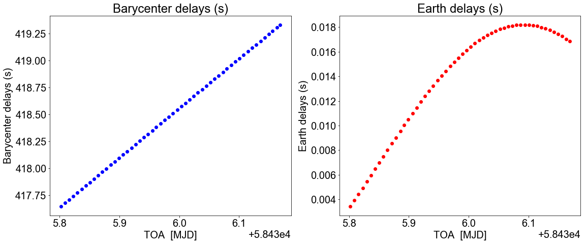
The barycenter delay was calculated by using the interpolated values from Section 4.4. The barycenter delay was calculated through the formula
\begin{equation} B_\mathrm{delay} = \frac{\underline{d} \cdot \underline{\hat{r}} }{c} \end{equation}
where $\underline{d}$ is the vector pointing from Earth to the barycenter, $\underline{\hat{r}}$ is the unit vector pointing from the barycenter to the pulsar and $c$ is the speed of light. The error on the vector pointing to the barycenter is hard to calculate exactly, but based on physical arguments, we have decided that it is negligible since the earth does not move very much around the barycenter in the span of 10 microseconds. Hence, the only source of error on the barycenter delay comes form the error on the unit vector. This was calculated and proved neglibile as well. Thus, we concluded that the error on the barycenter delay is negligible as well, for the purposes of this experiment. A figure showing the barycenter delays for the first measurement of the Crab pulsar is shown in Figure 1. The detailed code where the exact numbers and errors appear is available in the Downloads section.
The periods of the Crab and four other pulsars were calculated. First, an estimated period was considered. In the case of the Crab pulsar, this estimated period was generated using a program provided by the demonstrators. Otherwise, it was taken from the lab script table since the periods quoted there are not very exact. Then, the remainders of the ToAs with respect to these guess periods were calculated in each case. A linear increase was observed as the ToAs increased, wrapping around periodically as presented in Slider 4.2. The correct period of the pulsar could be calculated from the slope of these lines through the formula
\begin{equation} T_\mathrm{true} = \frac{T_\mathrm{guess}}{1-m} \end{equation}
where $m$ is the slope of the lines in Slider 4.2.


These remainders were then fitted in two ways. Method 1 of fitting consisted of taking each “remainder line” individually. A much more accurate test of the precision of this method is to calculate the new remainders. The results of dividing the ToAs by the new period is presented in Slider 4.3.


Method 2 of fitting consisted of putting the “remainder lines” back to back and fitting them together. The results of this process are shown in Slider4.5.


As before, this method’s accuracy was also tested by plotting the new remainders. Therefore, the remainders of the ToAs divided by the period obtained through Method 2 is shown in Slider 4.6.


From these figures and knowing the conditions in which each measurement is taken, it is easy to tell that Method 2 is better for high quality mesurements, while Method 1 is better for lower quality ones. The period of each pulsar and the associated errors are presented in Table 4.1.
The period derivative could only be obtained for the Crab pulsar. This quantitiy was obtained through two different methods as well. The first method consists of taking the period and time difference between two subsequent measurements. Three measurements were taken within one week of each other. The period was calculated for each of these measurements and the results are available in Table 4.1. Each difference was divided by its corresponding times span and hence an approximation for the period derivative was obtained. The second method was based on a similar analysis as performed in finding the periods. The remainders obtained by dividing the ToAs by the correct period reveals how much the period derivative that we assume deviates from the true period derivative, as in Slider 4.6 for example. These remainders can be fitted with a second order polynomial. The slope of the second order term in the polynomial is related to the period derivative as
\begin{equation} \dot{P_\mathrm{t}} = \frac{\dot{P_\mathrm{g}}}{1-m} \end{equation}
where $m$ is the slope of the second order term in the quadratic polynomial fit, $\dot{P_t}$ is the true period derivative of the pulsar and $\dot{P_\mathrm{g}}$ is the guess period derivative of the pulsar. The fits in Method 2 are presented in Slider 4.6.


The values obtained through each method are presented in Table 4.2.
When replotting the remainders, this time correcting for the period derivative as well, one gets a sinusoidal graph. This is shown in Slider 4.7.


The tables summarize all the results obtained by the timing analysis. The period derivative and the period of the Crab Pulsar was used to calculate its minimum surface magnetic field and its age.
| Pulsar name | Period (seconds) | |
|---|---|---|
| Method 1 | Method 2 | |
| B0329+54 | 0.03375705(4) | 0.0337570584(1) |
| B1642-03 | 0.38771567(1) | 0.38771569(3) |
| B1933+16 | 0.35879058(3) | 0.358790498(7) |
| B2020+28 | 0.343445657(5) | |
| Crab (Week 1) | 0.033755409(4) | 0.03375540740(1) |
| Crab (Week 2) | 0.033755697(3) | 0.03375569661(1) |
| Crab (Week 3) | 0.033755950(3) | 0.03375595035(7) |
| Pulsar name | Period derivative | |
|---|---|---|
| Method 1 | Method 2 | |
| Crab (Week 1) | 4.21e-13 | 4.01e-13 |
| Crab (Week 2) | 4.17(3)e-13 | 4.02e-13 |
| Crab (Week 3) | 4.2e-13 | 4.03e-13 |
The approximate characteristic age of the Crab pulsar is $Age \approx 1273.85$ years.
The approximate surface magnetic field of the Crab pulsar is $B \approx 1.2 \times 10^8$ T.
Finally, the second period derivative was also calculated but only an approximate value could be obtained, which is $\approx -4.8 \times 10^{-21}$ s$^{-1}$.