University of Manchester | 3rd Year Laboratory
Unknown ‘periodic pulse’ searches having been crucial for pulsar surveys after the first discoveries at Cambridge and the Molonglo telescope at Australia. The two methods prevalant for searching pulsars are:
Periodogram Analysis: This method involves directly looking at a train of regularly spaced pules.
Fourier Analysis: This method involves looking at the Fourier transform of the time series spectrum.
Periodogram analysis requires high sensitivity to detect broad pulses with broad widths $w$, compared to narrow pulses showing high signal to noise ratio. The increase in the signal to noise ratio is given by a factor of $(P/2w)^{1/2}$. For this experiment, the Fourier analysis technique is chosen as it is computationally more economical than the periodogram analysis [2].
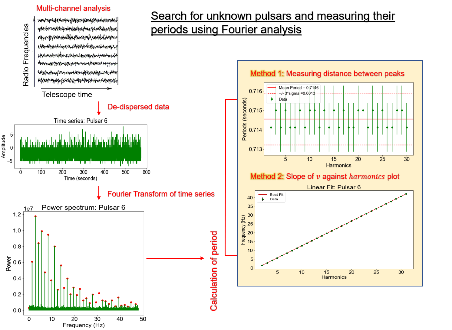
The data from a pulsar for a particular bandwidth is split into a number of independent frequency channels. This stored data is de-dispersed and the time series spectrum is obtained for the required integration time. The Fourier transform of the time series data stream is taken to precisely measure the period. Harmonics are a useful tool used for this measurement. Harmonics occur in the Fourier spectrum at integer multiples of the fundamental frequency. All periodic signals show harmonics. Figure 1 summarizes the Fourier trasform technique of measuring unkown pulsar periods.
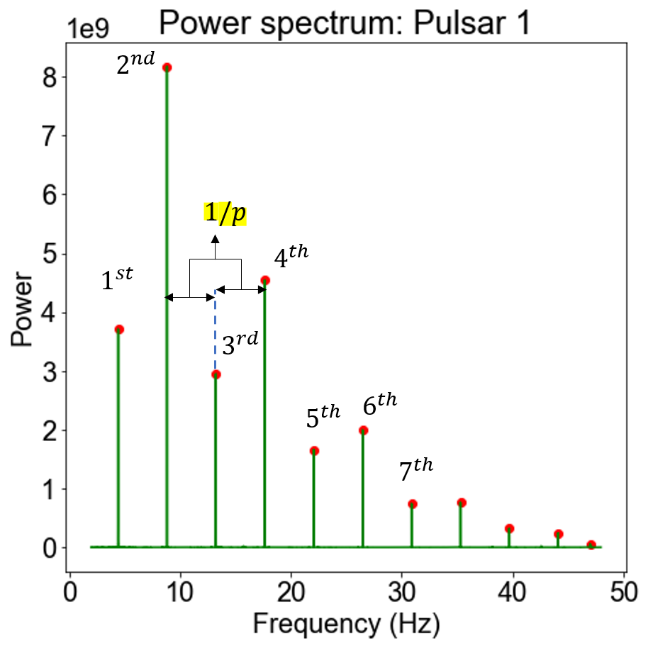
The $n^{th}$ harmonic has a frequency $v_n = Nv$ where $N$ is the total number of harmonics and $v$ is the fundamental frequency at which the first harmonic occurs, as shown in Figure 2. By definition, the period, $p$, is equal to $1/v$. Therefore, $p$ can be obtained from the information of the harmonics and the frequency at which they occur.
Six data streams of different pulsars, as measured by the 76-m Lovell telescope, were used for analysis. The de-dispersed time-series was plotted, as shown in Slider 3.1, and the time was calibrated on the x-axis by using the total integration time.


The discrete Fourier transform $\mathcal{F}$ (DFT) of each time series element ${\mathcal{T(j)}}$ was taken for the $N$ independently sampled data points. DFT of the $k^{th}$ component is given in the frequency domain $\mathcal{F}(k)\ \forall\ k, j\ \epsilon\ [0, N-1]$ is given as,
\begin{equation} \mathcal{F}(k) = \sum_{j=0}^{N-1} {\mathcal{T(j)}} {exp}^{-2i \pi jk/N} \end{equation}
where $i = \sqrt{-1}$. Each $\mathcal{F}(k)$ encodes the amplitude and phase of the sinusoid component ${exp}^{-2i \pi jk/N}$ of the ${\mathcal{T(j)}}$ element and has a frequency defined by $k/N$. The amplitude is given as,
\begin{equation} \mathcal{P}(k) = |\mathcal{F}(k)| = \sqrt{Re(\mathcal{F}(k))^2 + Im(\mathcal{F}(k))^2} \end{equation}
where $\mathcal{P}(k)$ is defined as the power. Slider 3.2 shows the Fourier transformed power spectrum of the time series elements for the 6 unknown pulsars which were plotted and shown in Slider 3.1. The width of each frequency bin is given as $1/\tau$ where $\tau$ is the total length of the observattion. It must be noted that $\tau = N t_{samp}$ where $t_{samp}$ is the sampling time. A periodic signal which is buried in noise in the time domain peaks with clarity in the frequency domain and becomes detectable [3].


Limitatiions in the DFT arise mainly due to non-uniform frequency responses which don’t match the bin centres. Additionally, the width of the bin limits the accuracy with which the peak can be measured. Hence, for all further use, the uncertainty in the frequency was quoted as the minimum resolution of the bins. Few power spectrums were dominated purely by noise at large freuencies, and hence, those frequencies were eliminated.
The peak frequency values in each power spectrum were noted for the 6 values. The harmonic number of each peak was incremented in steps of one. However, major radio interference contributions due to AC domestic currents were observed at multiples of 50 Hz. These frequencies were eliminated to avoid biases in the analysis. Accordingly, the harmonic number had to be corrected to compensate for the lost signal peak in the noise frequency ranges (50 Hz, 100 Hz, 150 Hz, etc.) due to AC currents as shown in Slider 3.3.


The peak frequencies were plotted as a function of the corrected harmonics. A linear model was applied on the data and the residual plots were used as a test to determine the goodness of the fit, as shown in Slider 3.4. The outlier points arising due to radio interference were easily detected and eliminated. The distribution of the data points shown in the residual plots are consistent with the linear model however, they show a systematic trend. The trend displays the limitation arising due to the finite frequency bin width. The trend can be understood as the carry-over or shift of the peak frequency. This is due to the increments in the amplitude being carried forward to the successive bins. When the increments are of comparable size to the width of the bin, it gets pushed in the successive bin.


The slope of the line is equal to $1/p$ as explained in Section 3.2. A weighted fit was performed with the weighs determined by the frequncy bin width. However, the error estimate obtained from the covariance matrix of the best-fitting line were small and unphysical. Hecnce, the successive approach detailed in Section 3.6 was used to obtain physical uncertainties on the period and to check the consistency of the calculated periods.
This method involved calculation of the distance between successive peaks in the power spectrum. The distance is equal to,
$1/p = f_{peak(i+1)} - f_{peak(i)}$, where $f_{peak(i)}$ is the peak frequncy of the $i^{th}$ harmonic. The uncertainties on the $f_{peak(i)}$ arising due to the finite sampling rate or bin width are propogated to obtain the uncertainties in $p_i$, as shown in the plots in Slider 3.5. The plot of the period as a function of the harmonic number centres about the true period of the pulsar. The standard deviation was used to obtain a physical uncertainty on the mean period. The values obtained using this method are consistent with those obtained from the slope of the frequncy vs harmonic plots, as detailed in Section 3.5.


The final results have been quoted in Table 3.1. The corresponding pulsar names for the calculated periods were found from the ‘Catalog of 558 Pulsars’ published by J.H. Taylor, R. N. Manchester and A. G. Lyne [4].
| Pulsar Data | Period (seconds) |
Width (ms) |
Pulsars |
|---|---|---|---|
| Pulsar 1 | 0.2265 ± 0.0002 | ~ 11 | B1929+10 |
| Pulsar 2 | 0.189 ± 0.003 | ~ 2 | B1821-19 |
| Pulsar 3 | 0.476 ± 0.001 | ~ 11 | B0626+24 |
| Pulsar 4 | 0.7397 ± 0.003 | ~ 19 | B1508+55 |
| Pulsar 5 | 0.2990 ± 0.001 | ~ 6 | B1702-19 |
| Pulsar 6 | 0.7146 ± 0.001 | ~ 12 | B0329+54 |