University of Manchester | 3rd Year Laboratory
Pulsars are relatively weak radio sources due to their small size. They usually emit their largest intensity at low radio frequencies around 400 MHz. However, at such frequencies, the pulses suffer from propagation effects when they travel through the interstellar medium [4].
The phenomenon is quantified in a term called the Dispersion Measure (DM). The DM is important in pulsar astronomy since it is one of the most fundamental properties such a celestial body [5]. Furthermore, once measured, the dispersion measure of a pulsar can be used to approximate the distance to that pulsar [6,7].
For an electromagnetic (EM) wave of frequency $\nu$ emitted at a discance $d$ from the observer and propagating through an electron plasma with uniform density $n_e$, the travel time of a pulse is \begin{equation} t_p = \frac{d}{c} + \frac{e^2}{2\pi m_e c}\frac{\int_{0}^{d} n_e dl}{\nu^2}. \end{equation} Therefore, the time delay is expressed as \begin{equation} t_d = 4150 \times\frac{DM}{\nu^2} \hspace{0.5em}\mathrm{s} \end{equation} where $DM$ is the disperion measure in $\mathrm{cm}^{-3}\mathrm{pc}$, or the integrated column density of free electrons along the line of sight [1].
Thus, it can be seen that the speed at which an electromagnetic wave propagates through the medium depends on its frequency. A pulsar source emits an EM pulse composed of several different frequencies. The intervening interstellar medium causes lower frequencies to travel more slowly. Thus, if we are observing a pulsar signal, we will see the higher frequencies arrive at us first, followed by the lower frequencies [2]. The light is dispersed by the ISM.
In this view, the dispersion measure is simply a constant of proportionality relating the frequency of the light to the extra amount of time (relative to vacuum) required to reach the observer due to dispersion. It depends on two quantities: the (electron) number density $n_e$ and the path length through the medium $d$ [1]. For example, a large DM value would tell us that the source is either relatively nearby but is traveling through a dense plasma, or it is far away, and traveling through a relatively less dense plasma. A visual representation of this process is shown in Figure 2.1.
To get an idea of the range in which one should find the $DM$ of a certain pulsar, 2D histograms were plotted. The scipy.optimize.minimize algorithm was used to find the $DM$ at which the intensity of the integrated profiles in Slider 2.2 peaked the highest. Five hundred initial values in the range of 0-200 were provided in each case, and the minimizer would always fall around the true value of the $DM$. An animation of this process is given in Figure 2.2.
From the final frames of the animation, one can see that the value of the $DM$ for the considered pulsar lies between 25 and 30. This represents a good check for the further results. On this page, we only present the animation for pulsar B0329+54, but animations for each analysed pulsar are found in the Downloads section.
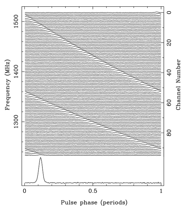
Ten pulsars were observed in the experiment using the 42-ft radio telescope, as detailed in Table 2.1. The Dispersion measure of each observed pulsar was calculated. The raw data for every considered pulsar is shown in Slider 2.1.


This raw data was then processed using three methods to get the dispersion measure. Essentialy, the right dispersion measure is obtained when the green line in the above plots sits vertically straight. The integrated profile (integrating over frequency) corresponding to each of the raw data plots is presented in Slider 2.2


In the following section we detail these methods, along with the results obtained for each pulsar.
This method consists of trying a range of DMs and plotting a graph of the corresponding integrated profile peaks. A peak is defined by the maximum y value of a figure from Slider 2.2. The DMs are sequentially applied to the raw data which results in systematic rotations of the green line in Slider 2.1. When the green line sits exactly vertical, the maximum signal to noise is achieved, the dispersion measure is correct and the value of the integrated profile peak is at a maximum. Graphs of the peaks against DMs of every pulsar are presented in Slider 2.3.


A polynomial fit was applied to all pulsars except the Crab B0531+21. For the Crab pulsar, a sum of gaussians was fitted to calculate the maximum of the $DM$ curve. The goodness of each fit was judged by the residual plot. The uncertainty bounds on each measured $DM$ was decided by chosing the points which lied at $97\%$ of the maxima on either sides. All pulsar DM values obtained this way, with their associated uncertainties, are presented in Table 2.1.
Each frequency channel (row) of the Slider 2.1 is considered separately. Slider 2.4 shows a visual representation of this for every pulsar we analysed i.e. plots the pulse profile for every frequency channel.


The grids in Slider 2.4 were filtered to only include rows which present a distinguishable peak. The time coordinate of each peak was then recorded. These times correspond to the times in the left hand side of Equation (2). Therefore, this could be plotted against the inverse squared frequency, times the constant 4150 (dispersion constant) to obtain a straight line. The straight line was then fitted with a linear model to obtain the dispersion measure, as obvious from Equation (2). Figures of these fits for each pulsar are presented in Slider 2.5.


Initially, the FWHM of every peak was calculated and that was considered as the error on the times in the above slider. However, it was immediately apparent that the errors were to large and unphysical. Hence, the width of a frequency bin was considered to be the error on these points instead.
The DMs obtained from each of these fits together with their associated errors (taken from the error on the slope of the fitted line) are presented in Table 2.1.
The final and most elegant method applied for calculating the $DM$ was performed by simulating 100 data sets by adding noise to the measured data. Each of these data sets are equally likely to be measured and the $DM$ was calculated for each of them. The following section details the methodology used to execute the analysis.
In order the add noise to the measured data, the nature of the white noise in the data was studied. As shown in Figure 2.2, the standard deviation in the noise was calculated in the integrated profile for each pulsar.
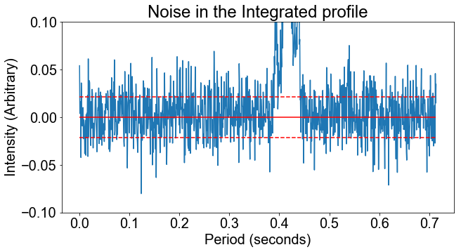
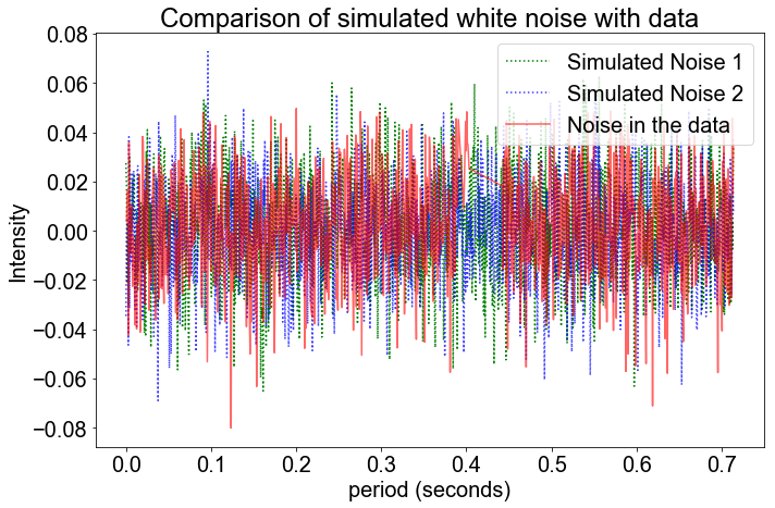
By understanding the nature of the white-noise, new noise data sets were simulated. As shown in Figure 2.3, the simulated data sets resemble the white noise in the measured data (shown in red) very closely.
100 such noise data sets were generated for each pulsar and added to the measured integrated profile data for each pulsar, which were shown in Slider 2.2. This generated 100 simulated signal data sets of which 2 arbitary sets are shown in Slider 2.6. As detailed in Method 1 in section 2.4.1, each data set was fitted with a polynomial function, or a sum of Gaussian functions in case of the Crab Pulsar, and the $DM$ was calculated. The calculated $DM$ for for all the 100 data sets was stored in an array and the mean $DM$ was measured. The uncertainty was quoted as the standard deviation in the obtained $DM$ values.


All the results obtained using this method have been states in Table 2.1.
The results of the dispersion measure obtained using the three methods are stated below.
| Pulsar Names | Dispersion Measure | ||
|---|---|---|---|
| Fitting the curve | Fitting the spectrum | Monte Carlo | |
| B0329+54 | 25.6757 ± 3.2703 | 29.473 ± 2.489 | 26.0490 ± 0.3591 |
| B0531+21(i) | 55.5045 ± 1.1892 | 55.834 ± 0.410 | 55.6937 ± 0.0946 |
| B0531+21(ii) | 55.8018 ± 1.1892 | 55.656 ± 0.238 | 55.8819 ± 0.0805 |
| B0531+21(iii) | 56.0000 ± 1.3874 | 55.725 ± 0.385 | 55.9550 ± 0.0762 |
| B1642-03 | 33.3063 ± 6.1441 | 32.434 ± 1.379 | 32.0871 ± 0.4578 |
| B1929+10 |
RFI | 1.6116 ± 0.8074 | |
| B1933+16 | 150.9510 ± 7.4074 | 158.009 ± 7.981 | 151.1997 ± 1.5803 |
| B2016+28 |
RFI | 1.4712 ± 3.4911 | |
| B2020+28 | 22.7027 ± 2.1802 | 20.061 ± 3.532 | 23.3594 ± 0.4248 |
| B2111+46 | 98.6486 ± 3.4034 | too noisy | 98.3332 ± 21.4281 |
The distance to the pulsar was estimated with the obtained values of $DM$ from Table 1.1. As stated in Eqn. 1, an electron density model needs to be assumed in order to calculate the distance. Generally, the mean Galactic electron density $n_e$ is the assumed to be $0.03\ cm^{-1}$. However, a more through approach was adopted for calculating the distance to pulsars using the two models detailed below:
First, the NE2001 model developed by Corder-Lazio [6] was applied. The model develops on the understanding of the ISM based on various measurements in the radio and x-ray band. By using 112 independedntly measured pulsar distances and scattering measures (SMs), the model successfully predicts large scale fluctuations (which cause scattering) and the smooth $n_e$ distribution. It also adds clumps and voids towards the pulsar based on the measured $DM$ values.
The YMW16 model developed by Yao, Manchester and Wang [7] was also attempted. The model is built on the NE2001, however, has some differences. For example, the four-armed spiral pattern of the Galaxy is considered. It also considers many local features in the galaxy like the Local Bubble (LB), enhances regions of $n_e$ at the edges of the LB, etc. It additionally, discards prior SMs measurements and does not assume any clump or void formations based on $DM$ values.
Table 2.2 shows the final results obtained using the measured $DM$ values from the Monte-Carlo method and using the NE2001 and YMW16 models respectively.
| Pulsar Names | Distance (kpc) | |
|---|---|---|
| Cordes-Lazio NE2001 (electron density model 1) |
YMW16 (electron density model 2) |
|
| B0329+54 | 1.088 ± 0.147 | 1.162 ± 0.116 |
| B0531+21(i) | 1.709 ± 0.298 | 1.282 ± 0.128 |
| B0531+21(ii) | 1.714 ± 0.299 |
1.286 ± 0.127 |
| B0531+21(iii) | 1.715 ± 0.298 | 1.287 ± 0.129 |
| B1642-03 | 1.057 ± 0.198 | 0.973 ± 0. 098 |
| B1933+16 | 5.484 ± 0.803 | 4.231 ± 0.423 |
| B2020+28 | 2.004 ± 0.389 | 1.617 ± 0.162 |
| B2111+46 | 3.890 ± 0.458 | 3.646 ± 0.365 |
The distances $d$ calculated using YMW16 for PSR B0329+54, B0531+21, B1933+16, B2020+28, and B2111+46 are consistent with accepted values quoted in the ATNF Pulsar Catalogue [8].
However, $d$ to B1642-03 shows consistency with the accepted value ($DM = 35.76\ pc\ cm^{-3}$, $d = 1.3\ kpc$) only when the NE2001 model was used to calculate $d$, the value obtained using YMW16 is inconsistent with the accepted value [8].